# List of packages you want to install
packages <- c("tidyverse", "data.table", "BEDMatrix", "Rfast", "susieR", "coloc")

# Function to check and install any missing packages
check_and_install <- function(pkg){
  if (!require(pkg, character.only = TRUE)) {
    install.packages(pkg, dependencies = TRUE)
    library(pkg, character.only = TRUE)
  }
}

# Use the function to check and install packages
sapply(packages, check_and_install)Transcriptome QGT Training 2023
Goals of Lab
- Predict whole blood expression from genotype
- Check how well the prediction works with GEUVADIS expression data
- Run association between predicted expression and a phenotype
- Calculate association between expression levels and coronary artery disease risk using s-predixcan
- Fine-map the coronary artery disease gwas results using torus
- Calculate colocalization probability using fastenloc
- Run cTWAS (fine-map SNPs and genes jointly)
Inital Remarks
- We ask you to actively participate in today’s hands on activities.
Note
Notice that we may ask you to share your screen for pedagogic purposes.
Send Haky a private message if you really don’t want to be called to share your screen.
If you have any concerns about this, please ask me or one of the TAs for assistance. We are here to help you learn.
Open the questionnaire forms at the beginning of each section and answer the questions as you go along
- Name is a mandatory field. You can use your name or a pseudonymn. Just keep using the same name for each submission
- We will ask you to submit partial set of answers so that we can get a sense of where people are
Through out the lab you will see code chucks that are written with bash, eval=FALSE in place of R. These chunks are meant to be run in your Rstudio terminal and not in the Rmarkdown file itself.
R code chunks also have “eval=FALSE”. When you click on the green triangle, the code will run in the R console but not when we knit the document. This just happened to be more convenient for us to generate a knitted html.
Set Up
Questionnaire 01
library(tidyverse)

## packages needed for susie+coloc
library(data.table)
library(BEDMatrix)
library(Rfast)
library(susieR)
library(coloc)
##library(tidyverse)cd "/cloud/project/"conda activate imlabtoolsprint(getwd())
lab="/cloud/project/QGT-Columbia-HKI-repo/"
CODE=glue::glue("{lab}/code")
source(glue::glue("{CODE}/load_data_functions.R"))
source(glue::glue("{CODE}/plotting_utils_functions.R"))
PRE="/cloud/project/QGT-Columbia-HKI-repo/box_files"
MODEL=glue::glue("{PRE}/models")
DATA=glue::glue("{PRE}/data")
RESULTS=glue::glue("{PRE}/results")
METAXCAN=glue::glue("{PRE}/repos/MetaXcan-master/software")
FASTENLOC=glue::glue("{PRE}/repos/fastenloc-master")
# This is a reference table we'll use a lot throughout the lab. It contains information about the genes.
gencode_df = load_gencode_df()MODEL
DATAexport PRE="/cloud/project/QGT-Columbia-HKI-repo/box_files"
export LAB="/cloud/project/QGT-Columbia-HKI-repo/"
export CODE=$LAB/code
export DATA=$PRE/data
export MODEL=$PRE/models
export RESULTS=$PRE/results
export METAXCAN=$PRE/repos/MetaXcan-master/software
echo $CODE
echo $RESULTS
Transcriptome-wide association (Review)
Now we will perform a transcriptome-wide association analysis using the PrediXcan suite of tools. 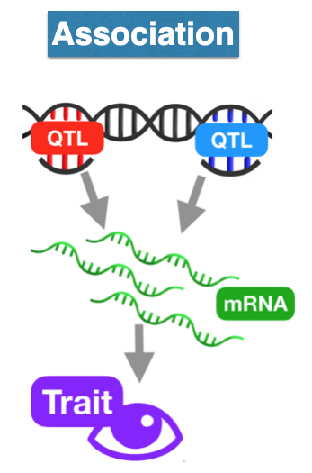
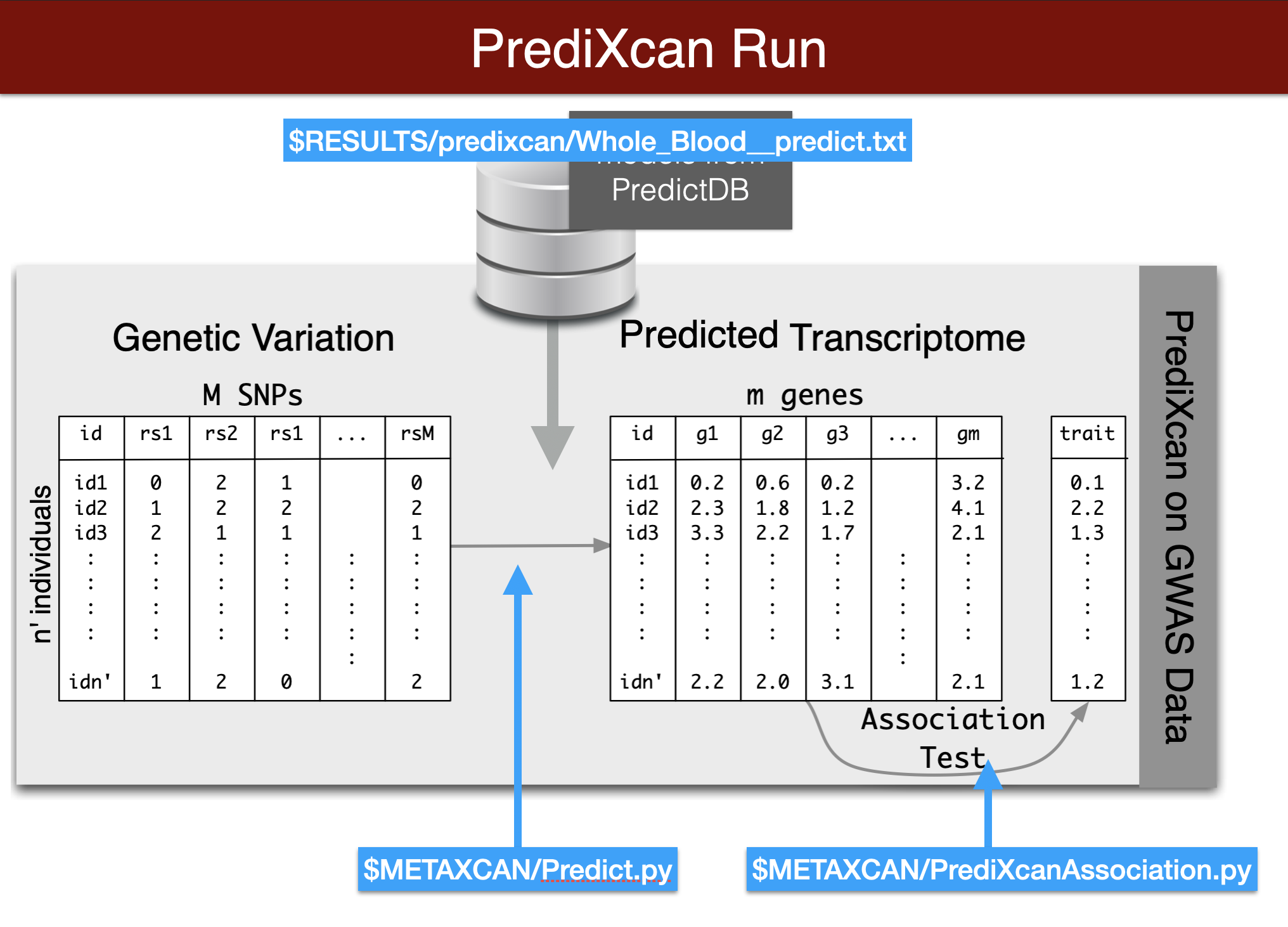
We start by predicting the expression levels of genes using the genotype data and the prediction weights and then perform an association between the predicted expression and the phenotype (denoted trait in the figure below).
Questionnaire 02
Predict Expression from genotype
In this section we will predict expression of genes in whole blood using the Predict.py code in the METAXCAN folder.
Prediction models (weights) are located in the MODEL folder. Additional models for different tissues and transcriptome studies can be downloaded from predictdb.org.
This run should take about one minute.
printf "Predict expression\n\n"
python3 $METAXCAN/Predict.py \
--model_db_path $PRE/models/gtex_v8_en/en_Whole_Blood.db \
--vcf_genotypes $DATA/predixcan/genotype/filtered.vcf.gz \
--vcf_mode genotyped \
--variant_mapping $DATA/predixcan/gtex_v8_eur_filtered_maf0.01_monoallelic_variants.txt.gz id rsid \
--on_the_fly_mapping METADATA "chr{}_{}_{}_{}_b38" \
--prediction_output $RESULTS/predixcan/Whole_Blood__predict.txt \
--prediction_summary_output $RESULTS/predixcan/Whole_Blood__summary.txt \
--verbosity 9 \
--throw
Note we are only predicting chromosome 22 here (check by running “predicted_expression %>% count(chromosome)” in the console)
Find additional information in this wiki
prediction_fp = glue::glue("{RESULTS}/predixcan/Whole_Blood__predict.txt")

## Read the Predict.py output into a dataframe. This function reorganizes the data and adds gene names.
predicted_expression = load_predicted_expression(prediction_fp, gencode_df)

head(predicted_expression)

## read summary of prediction, number of SNPs per gene, cross validated prediction performance
prediction_summary = load_prediction_summary(glue::glue("{RESULTS}/predixcan/Whole_Blood__summary.txt"), gencode_df)
## number of genes with a prediction model
dim(prediction_summary)
head(prediction_summary)

## how many unique genes were predicted?
predicted_expression %>% .[["gene_id"]] %>% unique() %>% length()

## gene expression were predicted for how many people?
predicted_expression %>% .[["IID"]] %>% unique() %>% length()

print("distribution of prediction performance r2")
summary(prediction_summary$pred_perf_r2)
hist(prediction_summary$pred_perf_r2)
## Note: this is what the prediction trainer reported as prediction performance
(Optional) Assess Actual Prediction Performance
## download and read observed expression data from GEUVADIS
## from https://uchicago.box.com/s/4y7xle5l0pnq9d1fwmthe2ewhogrnlrv

obs_exp<- read_csv(glue::glue("{DATA}/predixcan/GEUVADIS.observed_df.csv.gz"))

## Note that the version of the ensemble id of the gene was removed
head(predicted_expression)

## Q: how many genes were predicted?
length(unique(predicted_expression$gene_id))

## inner join predicted expression with observed expression data (by IID and gene)
## common errors occur when ensemble id's have versions in one set and not the other set
fullset=inner_join(predicted_expression, obs_exp, by = c("gene_id","IID"))

## calculate spearman correlation for all genes
genelist = unique(predicted_expression$gene_id)
corvec = rep(NA,length(genelist))
names(corvec) = genelist
for(gg in 1:length(genelist))
{
  ind = fullset$gene_id==genelist[gg]
  corvec[gg] = cor(fullset$predicted_expression[ind], fullset$observed_expression[ind])
}

## what's the best performing gene?

## plot the histogram of the prediction performance
hist(corvec)

## list the top 10 best performing genes
head(sort(corvec,decreasing = TRUE),2)
tail(sort(corvec,decreasing = TRUE),2)

## plot the correlation of the top 2 best performing genes bottom 2

geneid = "ENSG00000100376"
genename = gencode_df %>% filter(gene_id==geneid) %>% .[["gene_name"]]
fullset %>% filter(gene_id==geneid) %>% ggplot(aes(observed_expression, predicted_expression))+geom_point()+ggtitle(paste(genename, "-",geneid))

geneid = "ENSG00000075234"
genename = gencode_df %>% filter(gene_id==geneid) %>% .[["gene_name"]]
fullset %>% filter(gene_id==geneid) %>% ggplot(aes(observed_expression, predicted_expression))+geom_point()+ggtitle(paste(genename, "-", geneid))

geneid = "ENSG00000070371"
genename = gencode_df %>% filter(gene_id==geneid) %>% .[["gene_name"]]
fullset %>% filter(gene_id==geneid) %>% ggplot(aes(observed_expression, predicted_expression))+geom_point()+ggtitle(paste(genename, "-", geneid))

geneid = "ENSG00000184164"
genename = gencode_df %>% filter(gene_id==geneid) %>% .[["gene_name"]]
fullset %>% filter(gene_id==geneid) %>% ggplot(aes(observed_expression, predicted_expression))+geom_point()+ggtitle(paste(genename, "-", geneid))
Run PrediXcan association
Questionnaire 03
We are going to use a simulated phenotype for which only UPK3A has an effect on the phenotype (\(\beta=-0.9887378\))
\(Y = \sum_k T_k \beta_k + \epsilon\)
with random effects \(\beta_k \sim (1-\pi)\cdot \delta_0 + \pi\cdot N(0,1)\)
export PHENO="sim.spike_n_slab_0.01_pve0.1"

printf "association\n\n"
python3 $METAXCAN/PrediXcanAssociation.py \
--expression_file $RESULTS/predixcan/Whole_Blood__predict.txt \
--input_phenos_file $DATA/predixcan/phenotype/$PHENO.txt \
--input_phenos_column pheno \
--output $RESULTS/predixcan/$PHENO/Whole_Blood__association.txt \
--verbosity 9 \
--throw
More predicted phenotypes can be found in $DATA/predixcan/phenotype/. The naming of the phenotypes provides information about the genetic architecture: the number after pve is the proportion of variance of Y explained by the genetic component of expression. The number after spike_n_slab represents the probability that a gene is causal π (i.e. prob β≠0)
Looking at Association Results
## read association results
PHENO="sim.spike_n_slab_0.01_pve0.1"

predixcan_association = load_predixcan_association(glue::glue("{RESULTS}/predixcan/{PHENO}/Whole_Blood__association.txt"), gencode_df)

## take a look at the results
dim(predixcan_association)
predixcan_association %>% arrange(pvalue) %>% select(gene_name,effect,se,pvalue,gene) %>% head
predixcan_association %>% arrange(pvalue) %>% ggplot(aes(pvalue)) + geom_histogram(bins=10)
## compare distribution against the null (uniform)
gg_qqplot(predixcan_association$pvalue, max_yval = 40)
Comparing the Estimated Effect Size with True Effect Size
truebetas = load_truebetas(glue::glue("{DATA}/predixcan/phenotype/gene-effects/{PHENO}.txt"), gencode_df)
betas = (predixcan_association %>%
               inner_join(truebetas,by=c("gene"="gene_id")) %>%
               select(c('estimated_beta'='effect',
                        'true_beta'='effect_size',
                        'pvalue',
                        'gene_id'='gene',
                        'gene_name'='gene_name.x',
                        'region_id'='region_id.x')))
betas %>% arrange(pvalue) %>% select(gene_name,estimated_beta,true_beta,pvalue) %>% head
## do you see examples of potential LD contamination?
betas %>% mutate(causal= true_beta!=0) %>% ggplot(aes(estimated_beta, true_beta,col=causal))+geom_point(alpha=0.6,size=5)+geom_abline()+theme_bw()
UPK3A is the causal gene and has the most significant pvalue. RIBC2 is also significantly associated but has no causal role (we know because we simulated the phenotype that way). Why?
Hint: correlation between the genes
Run Summary PrediXcan
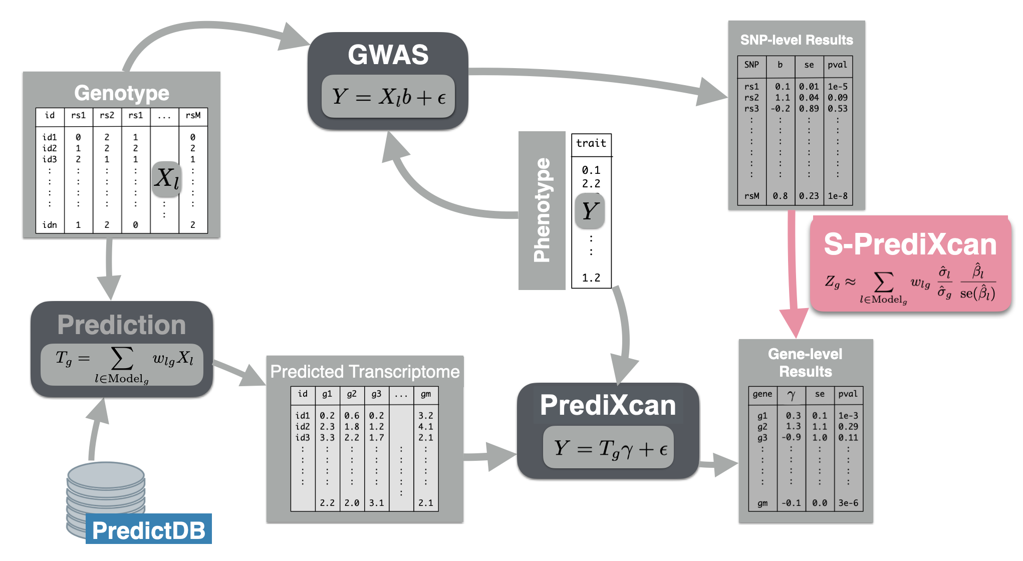
Now we will use the summary results from a GWAS of coronary artery disease to calculate the association between the genetic component of the expression of genes and coronary artery disease risk. We will use the SPrediXcan.py.
The GWAS results (harmonized and imputed) for coronary artery disease are available in $PRE/spredixcan/data/
Questionnaire 04
Running S-PrediXcan
python $METAXCAN/SPrediXcan.py \
--gwas_file  $DATA/spredixcan/imputed_CARDIoGRAM_C4D_CAD_ADDITIVE.txt.gz \
--snp_column panel_variant_id \
--effect_allele_column effect_allele \
--non_effect_allele_column non_effect_allele \
--zscore_column zscore \
--model_db_path $MODEL/gtex_v8_mashr/mashr_Whole_Blood.db \
--covariance $MODEL/gtex_v8_mashr/mashr_Whole_Blood.txt.gz \
--keep_non_rsid \
--additional_output \
--model_db_snp_key varID \
--throw \
--output_file $RESULTS/spredixcan/eqtl/CARDIoGRAM_C4D_CAD_ADDITIVE__PM__Whole_Blood.csv
We can run the full genome because the summary statistics based PrediXcan is much faster than individual level one.
Plot and Interpret Results
spredixcan_association = load_spredixcan_association(glue::glue("{RESULTS}/spredixcan/eqtl/CARDIoGRAM_C4D_CAD_ADDITIVE__PM__Whole_Blood.csv"), gencode_df)
dim(spredixcan_association)
spredixcan_association %>% arrange(pvalue) %>% head
spredixcan_association %>% arrange(pvalue) %>% ggplot(aes(pvalue)) + geom_histogram(bins=20)

gg_qqplot(spredixcan_association$pvalue)
Question: SORT1, considered to be a causal gene for LDL cholesterol and as a consequence of coronary artery disease, is not found here. Why?
Run S-PrediXcan using gene expression predicted in liver
-[] Run s-predixcan with liver model, do you find SORT1? Is it significant?
#loction Liver models
#/cloud/project/QGT-Columbia-HKI-repo/box_files/models/gtex_v8_mashr/
python $METAXCAN/SPrediXcan.py \
--gwas_file  $DATA/spredixcan/imputed_CARDIoGRAM_C4D_CAD_ADDITIVE.txt.gz \
--snp_column panel_variant_id \
--effect_allele_column effect_allele \
--non_effect_allele_column non_effect_allele \
--zscore_column zscore \
--model_db_path $MODEL/gtex_v8_mashr/mashr_Liver.db \
--covariance $MODEL/gtex_v8_mashr/mashr_Liver.txt.gz \
--keep_non_rsid \
--additional_output \
--model_db_snp_key varID \
--throw \
--output_file $RESULTS/spredixcan/eqtl/CARDIoGRAM_C4D_CAD_ADDITIVE__PM__Liver.csvspredixcan_association_L= load_spredixcan_association(glue::glue("{RESULTS}/spredixcan/eqtl/CARDIoGRAM_C4D_CAD_ADDITIVE__PM__Liver.csv"), gencode_df)
dim(spredixcan_association_L)
spredixcan_association_L %>% arrange(pvalue) %>% head
spredixcan_association_L %>% arrange(pvalue) %>% ggplot(aes(pvalue)) + geom_histogram(bins=20)
gg_qqplot(spredixcan_association_L$pvalue)
col_order= c("gene_name","gene","zscore","effect_size","pvalue","var_g","pred_perf_r2", "pred_perf_pval","pred_perf_qval", "n_snps_used", "n_snps_in_cov", "n_snps_in_model","best_gwas_p","largest_weight")
spredixcan_association_L <- spredixcan_association_L[, col_order]
filter(spredixcan_association_L, gene_name=="SORT1")(Optional) Compare zscores in liver and whole blood.
Recall that zscore is the effect size divided by the standard error
spredixcan_association_L=rename(spredixcan_association_L, zscore_liver = "zscore")
head(spredixcan_association_L)
test=left_join(spredixcan_association, spredixcan_association_L, by="gene_name")
test=select(test,"gene_name","zscore","zscore_liver")
test %>% arrange(zscore_liver) %>% head

test %>% mutate(zscore_WB=zscore) %>% ggplot(aes(zscore_WB,zscore_liver)) + geom_point(size=3,alpha=.6) + geom_abline()

## S-PrediXcan association in liver and whole blood are significantly correlated
cor.test(test$zscore,test$zscore_liver)
(Optional) Run MultiXcan
multixcan aggregates information across multiple tissues to boost the power to detect association. It was developed movivated by the fact that eQTLs are shared across multiple tissues, i.e. many genetic variants that regulate expression are common across tissues.
before you run multixcan ensure you have run s-predixcan for all the tissues you want to multixcan. In this tutorial we have two tissues (liver and whole blood), ensure you have run s-predixcan with the two tissues before running multixcan.
One thing to note is to ensure similar naming pattern for the output files. This is to ensure the files are captured correctly when running multixcan’s filter.
python $METAXCAN/SMulTiXcan.py \
--models_folder $MODEL/gtex_v8_mashr \
--models_name_pattern "mashr_(.*).db" \
--snp_covariance $MODEL/gtex_v8_expression_mashr_snp_smultixcan_covariance.txt.gz \
--metaxcan_folder $RESULTS/spredixcan/eqtl/ \
--metaxcan_filter "CARDIoGRAM_C4D_CAD_ADDITIVE__PM__(.*).csv" \
--metaxcan_file_name_parse_pattern "(.*)__PM__(.*).csv" \
--gwas_file $DATA/spredixcan/imputed_CARDIoGRAM_C4D_CAD_ADDITIVE.txt.gz \
--snp_column panel_variant_id --effect_allele_column effect_allele --non_effect_allele_column non_effect_allele --zscore_column zscore --keep_non_rsid --model_db_snp_key varID \
--cutoff_condition_number 30 \
--verbosity 9 \
--throw \
--output $RESULTS/smultixcan/eqtl/CARDIoGRAM_C4D_CAD_ADDITIVE_smultixcan.txt
Colocalization Methods (Review)
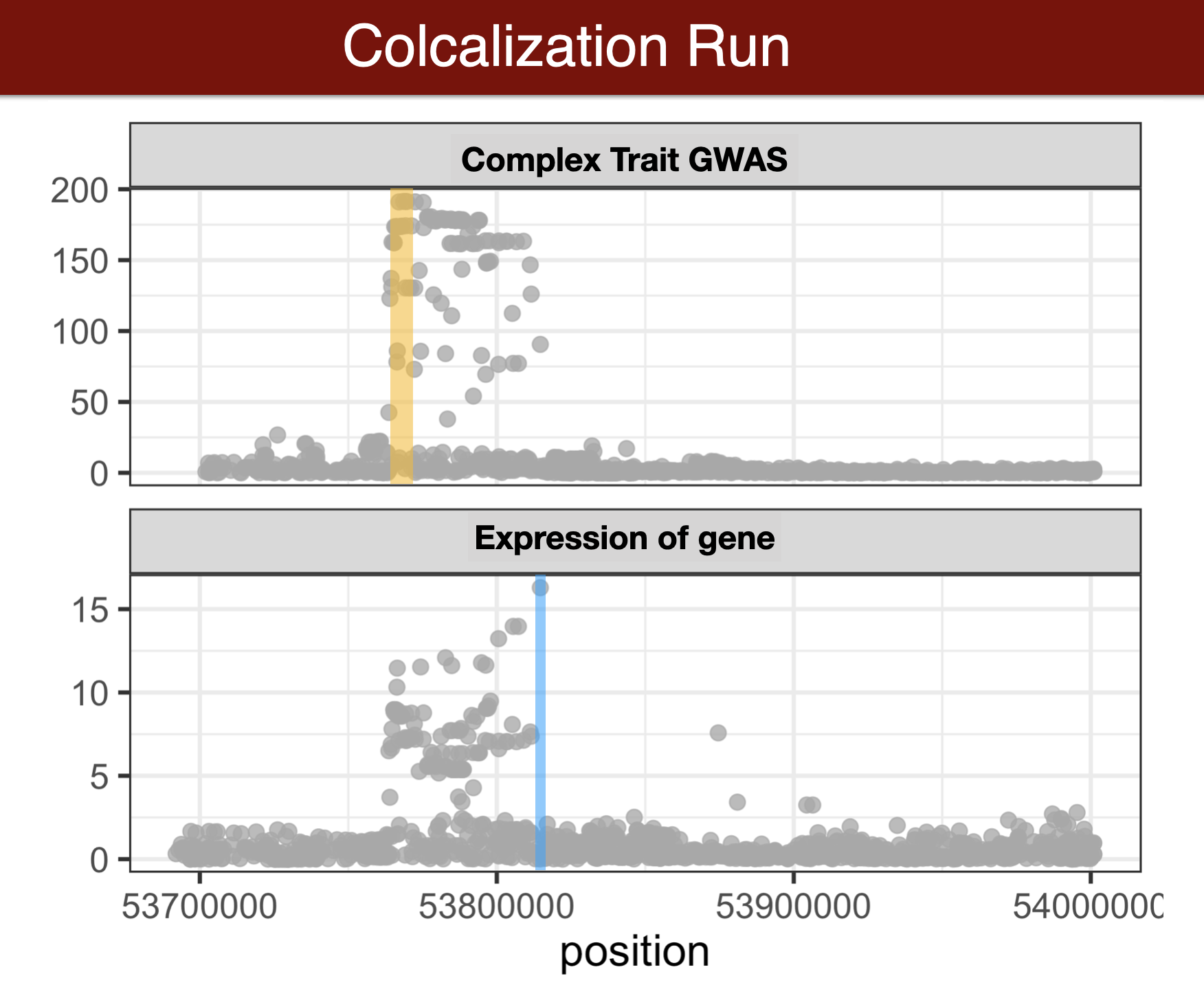
Colocalization methods seek to estimate the probability that the complex trait and expression causal variants are the same. We favor methods that calculate the probability of causality for each trait (posterior inclusion probability), called fine-mapping methods. Here we use susie for fine-mapping and coloc for colocalization.
Questionnaire 5
Run colocalization
When you use coloc on your own data, you may want to check out coloc’s documentation, with good advice and tips on avoiding common mistakes https://cran.r-project.org/web/packages/coloc/vignettes
Due to time constraints, we will run one region and one gene only
- Finemap GWAS of CAD
- Finemap eQTL of SORT1
For finemapping, we need the summary statistics (effect size, standard errors, etc) and the correlation between SNPs (LD matrix)
load the genotype to calculate the ld matrix
# load the genotype to calculate the ld matrix
X_mat <- BEDMatrix(glue::glue("{DATA}/colocalization/geuvadis_chr1"))
colnames(X_mat) <- gsub("\\_.*", "",colnames(X_mat))
colnames(X_mat) <- str_replace_all(colnames(X_mat),":","_")
snp_info <- fread(glue::glue("{DATA}/colocalization/geuvadis_chr1.bim")) %>%
  setnames(., colnames(.), c("chr", "snp", "cm", "pos", "alt", "ref"))

snp_info$snp <- str_replace_all(snp_info$snp,":","_")
Load the eqtl and gwas effect size files
# load the eqtl effect sizes
gene_ss <- fread(glue::glue("{DATA}/colocalization/Liver_chr1.txt"))

# load gwas effect sizes
gwas <- data.table::fread(glue::glue("{DATA}/spredixcan/imputed_CARDIoGRAM_C4D_CAD_ADDITIVE.txt.gz"))

# filter to select genome wide significant snps at 5 × 10⁻⁸
filtered_regions <- gwas %>% dplyr::filter(pvalue < 5e-8)

# load the ld block
ldblocks <-read_tsv(glue::glue("{DATA}/spredixcan/eur_ld.hg38.txt.gz"))
Find regions with the strongest signal in the gwas
# get the loci where the significant snps are located
for (n in 1:nrow(filtered_regions)){
  # extract genename, start and end
  variant_id <- as.character(filtered_regions[n,"variant_id"])
  variant_chr <- as.character(filtered_regions[n,"chromosome"])
  variant_pos <- as.numeric(filtered_regions[n,"position"])
  #gene_end <- as.numeric(genes[n,"end"])

  locus <- ldblocks %>%
    dplyr::filter(chr == variant_chr) %>%
    filter(variant_pos >= start & variant_pos < stop) %>%
    mutate(locus_name = paste0(chr,"_",start,"_",stop)) %>%
    dplyr::rename(locus_start=start,locus_end=stop) %>%
    mutate(variant_id = variant_id, position=variant_pos)

  # create a data frame with info
  if (exists('all_loci') && is.data.frame(get('all_loci'))) {
    all_loci <- rbind(all_loci,locus)
  } else {
    all_loci <- locus
  }
}

# select uniq loci
d_loci <- all_loci %>%
  dplyr::select(locus_name,chr,locus_start,locus_end) %>%
  dplyr::distinct()
select a region to run coloc
# select regions to fine map. we are going to use regions in chromosome 1
uniq_loci <- d_loci %>% dplyr::filter("chr1" == chr)
n = 3 # chr1_107867043_109761309 region

# extract information
l_chr = as.numeric(str_remove(uniq_loci[n,"chr"],"chr"))
s_chr = uniq_loci[n,]$chr
l_start = uniq_loci[n,]$locus_start
l_stop = uniq_loci[n,]$locus_end
l_name = uniq_loci[n,]$locus_name
Prepare gwas data for coloc
# select snps for the region from the summary stats
ss <- gwas %>%
  dplyr::filter(chromosome == s_chr) %>%
  dplyr::filter(position >= l_start & position <= l_stop) %>%
  dplyr::filter(! is.na(effect_size))

# find the snps in the genotype to calculate the correlation
g.snps <- ss %>% inner_join(snp_info %>% mutate(chr = glue::glue("chr{chr}")),
                            by=c("chromosome" = "chr","panel_variant_id" = "snp"))


# select genotype to calculate correlation
#f_mat <- X_mat[,g.snps$snp]
f_mat <- X_mat[,g.snps$panel_variant_id]

# calculate corr
R = cora(f_mat) # the package is for speed

## clean up
rm(f_mat)

ff <- g.snps %>% dplyr::filter(! is.na(effect_size)) %>% #select(-snp) %>%
  dplyr::rename(snp=panel_variant_id,beta=effect_size) %>%
  mutate(varbeta = standard_error^2) %>%
  dplyr::select(beta,varbeta,snp,position) %>% as.list()

ff$type <- "cc"
ff$sdY <- 1

ff$LD = R
ff$N = 184305

## check the data (NULL means it's fine)
check_dataset(ff)
Prepare eqtl data for coloc
#Using SORT1 gene and liver tissue
gene <- gene_ss %>% dplyr::filter(gene_id == "ENSG00000134243.11") %>%
  dplyr::rename(snp = variant_id,beta = slope, MAF = maf,
                pvalue = pval_nominal) %>%
  mutate(varbeta = slope_se^2, name = snp) %>%
  filter(! is.na(varbeta)) %>%
  separate(name, into = c("chr", "position","ref","alt","build"),sep = "_")

## calculate the ld matrix
### get the snps
gene.snps <- gene %>% mutate(position = as.integer(position)) %>%
  inner_join(snp_info %>% mutate(chr = glue::glue("chr{chr}")),
                              by=c("chr" = "chr","snp" = "snp"))

# select genotype to calculate correlation
g_mat <- X_mat[,gene.snps$snp]
# calculate corr
g.R = cora(g_mat)

# clean up
rm(g_mat)

# format data for coloc
gg <- gene %>% dplyr::filter(snp %in% gene.snps$snp) %>%
  mutate(position = as.integer(position)) %>%
  dplyr::select(beta,varbeta,snp,position,MAF, pvalue) %>% as.list()

gg$type <- "quant"
gg$LD = g.R
gg$N = 208 # 670 for blood

## check the data
check_dataset(gg)
run older version of coloc which assumes single causal variant
coloc.abf makes the simplifying assumption that each trait has at most one causal variant in the region under consideration
my.res <- coloc.abf(dataset1=ff, dataset2=gg)
sensitivity(my.res,"H4 > 0.9")
run coloc allowing multiple causal variants
Multiple causal variants, using SuSiE to separate the signals
# Run susie fine maooing
S3 = runsusie(ff)
S4 = runsusie(gg)
#summary(S3)

# Run coloc
susie.res=coloc.susie(S3,S4)
print(susie.res$summary)
SuSiE can take a while to run on larger datasets, so it is best to run once per dataset with the =runsusie= function, store the results and feed those into subsequent analyses.
plot the coloc result with the sensitivity function because weird effects are much easier to understand visually
sensitivity(susie.res,"H4 > 0.9",row=1,dataset1=ff,dataset2=gg,)cTWAS
cTWAS stands for causal TWAS and seeks to calculate the posterior inclusion probability of genes and SNPs in a given region to be causal. It’s a modification of SUSIER that adds predicted gene expression levels in addition to SNPs in the analysis. It is not yet published, but the authors (Siming Zhao, Wesley Crouse, Matthew Stephens et al) have shared a vignette with us to try it out.
Thank you, Wes, for creating this portion of the lab!
Questionnaire 06
#install.packages("R.utils")

#install.packages("remotes")
#remotes::install_github("simingz/ctwas", ref = "develop")

library(ctwas)

#get positions for region of interest (SORT1/PSRC1 locus)
region <- unlist(strsplit(spredixcan_association$region_id[spredixcan_association$gene_name=="PSRC1"], "_"))
chr <- region[2]
start <- as.numeric(region[3])
end <- as.numeric(region[4])

#format summary statistics (and subset to variants in region to save memory)
z_snp <- data.table::fread(glue::glue("{DATA}/spredixcan/imputed_CARDIoGRAM_C4D_CAD_ADDITIVE.txt.gz"), select=c("chromosome", "position", "variant_id", "effect_allele", "non_effect_allele", "zscore", "sample_size"))
z_snp <- z_snp[z_snp$chromosome==chr & z_snp$position >= start & z_snp$position <= end,]
z_snp <- z_snp[!is.na(z_snp$variant_id),-(1:2)]
colnames(z_snp) <- c("id", "A1", "A2", "z", "ss")

#specify directories for LD matrices and weights
ld_R_dir <- glue::glue("{DATA}/cTWAS/LD_matrices")
weight <-  glue::glue("{MODEL}/gtex_v8_mashr/mashr_Liver.db")

#specify output locations and names for cTWAS
outputdir <- glue::glue("{DATA}/cTWAS/results/")
outname.e <- "CARDIoGRAM_Liver_expr"
outname <- "CARDIoGRAM_Liver_ctwas"

#impute gene z scores using cTWAS and save the results
##################################
# NOTE: we are skipping this step and using the precomputed values
## takes ~10 minutes
##################################
# ctwas_imputation <- impute_expr_z(z_snp=z_snp, weight=weight, ld_R_dir=ld_R_dir, outputdir=outputdir, outname=outname.e, harmonize_z=F, harmonize_wgt=F)
# save(ctwas_imputation, file = paste0(outputdir, outname.e, "_output.Rd"))
load(paste0(outputdir, outname.e, "_output.Rd"))

z_gene <- ctwas_imputation$z_gene
ld_exprfs <- ctwas_imputation$ld_exprfs
z_snp <- ctwas_imputation$z_snp

#make custom region file for single region
ld_regions_custom <- data.frame("chr" = chr, "start" = start, "stop" = end)

write.table(ld_regions_custom,
            file= paste0(outputdir, "ld_regions_custom.txt"),
            row.names=F, col.names=T, sep="\t", quote = F)

ld_regions_custom <- paste0(outputdir, "ld_regions_custom.txt")

#run cTWAS with pre-specified prior parameters at a single locus
#estimating prior requires genome-wide data, too slow for demonstration
#prior is 1% inclusion for genes and is 100x more likely than SNPs
#prior assumes genes have larger effect size than SNPs, in reasonable range for data we've looked at
ctwas_rss(z_gene=z_gene, z_snp=z_snp, ld_exprfs=ld_exprfs, ld_R_dir = ld_R_dir, ld_regions_custom=ld_regions_custom, outputdir = outputdir, outname = outname, thin = 0.01,
          estimate_group_prior = F,
          estimate_group_prior_var = F,
          group_prior=c(0.01, 0.0001),
          group_prior_var=c(50, 25))

#load results
ctwas_results <- data.table::fread(paste0(outputdir,outname,".susieIrss.txt"))

#merge gene names into the results
sqlite <- RSQLite::dbDriver("SQLite")
db = RSQLite::dbConnect(sqlite, weight)
query <- function(...) RSQLite::dbGetQuery(db, ...)
extra_table <- query("select * from extra")
RSQLite::dbDisconnect(db)

ctwas_results$genename <- extra_table$genename[match(ctwas_results$id, extra_table$gene)]

#show results with highest PIPs
col_order_2= c("genename", "chrom", "id", "pos", "type", "region_tag1", "region_tag2", "cs_index", "susie_pip" , "mu2")
ctwas_results <- ctwas_results[, ..col_order_2]
head(ctwas_results[order(-ctwas_results$susie_pip),])
FAQ and frequent errors
conda environment may not load correctly after resuming the project in Rstudio cloud
when inner joining by ensemble id of genes, make sure that both datasets have either the same versions or remove versions
Contributors
- Festus Nyasimi
- Margaret Perry
- Wes Crouse
- Owen Melia