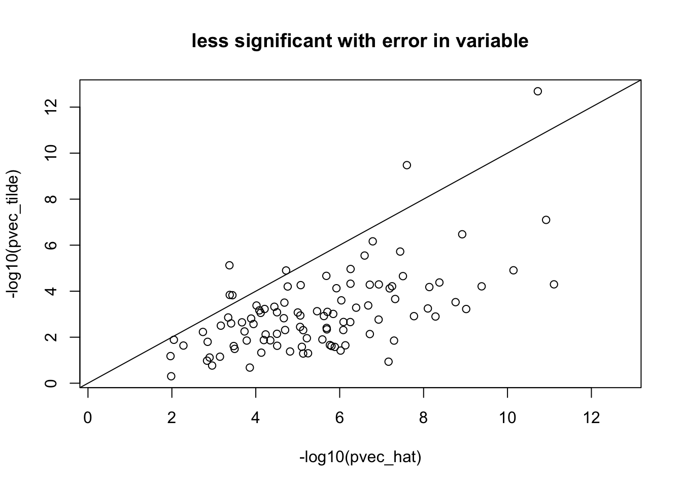
Uncertainty in predicted expression causes attenuation bias, and reduced significance of the association. Hence significance is underestimated.
PrediXcan seeks to test whether the genetically regulated expression levels (GReX=\(T_g\)) of a gene is associated with the phenotype of interest. However, in practice the the GReX is known only with some error. If the error in GReX is independent of the error in Y (\(\epsilon_Y\)) and the GReX, then
the test is valid
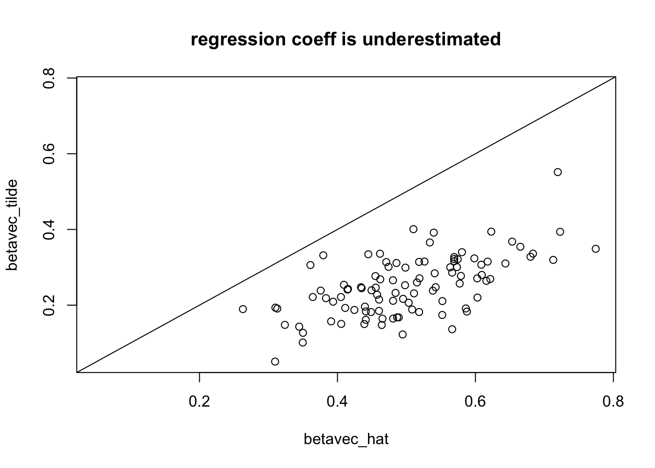
the estimated effect size of the GReX on the phenotype is biased towards zero (attenuation bias)
the power of the test, \(\beta=0\), is reduced
see Fuller, W. 1987 Measurement Error Models, Wiley & Sons pg.4.
Derivation of the attenuation
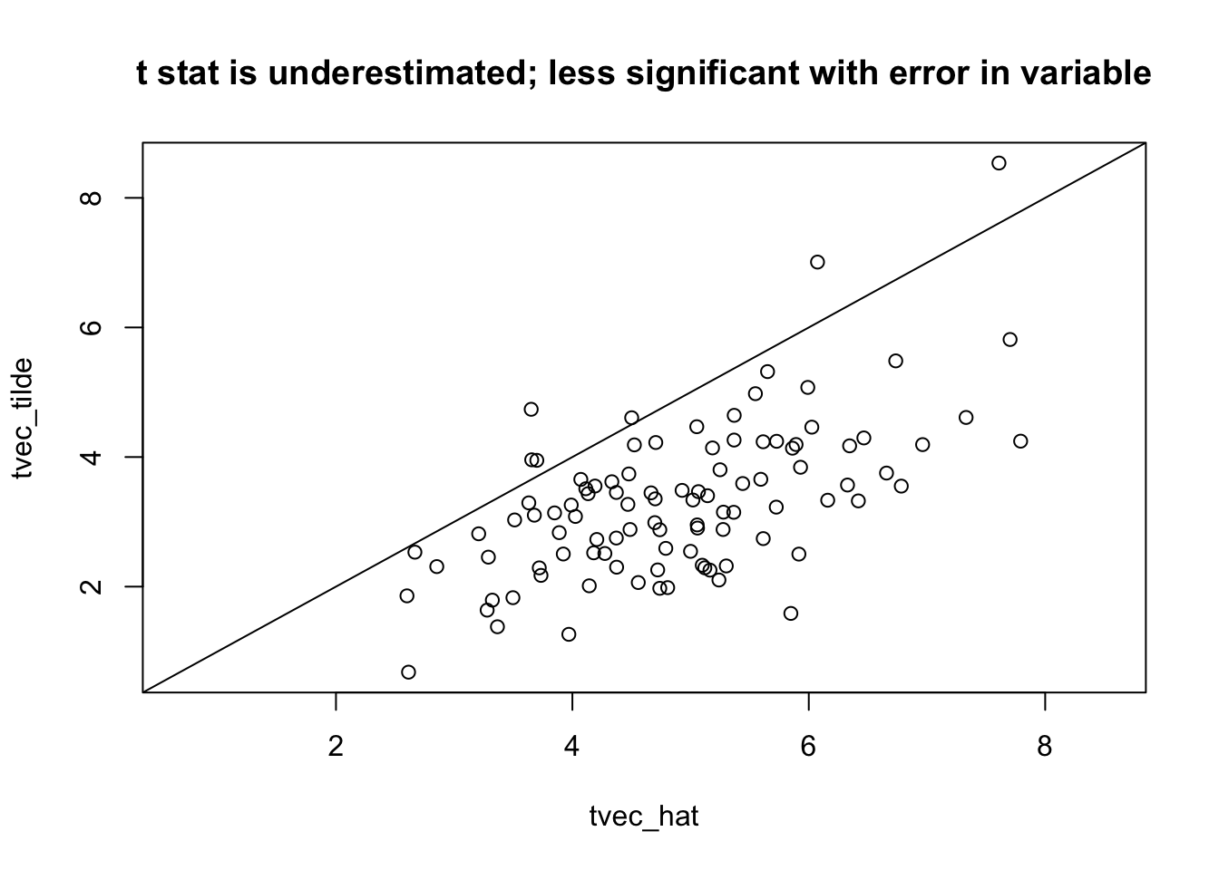
Below, I show that the estimate is attenuated (biased towards zero) and provide a link to the proof that the t statistic (estimated beta divided by its standard error when using the noisy \(=\tilde{T_g}\)) is lower, i.e. less significant.
Let us assume that the phenotype \(Y\) is a linear function of the genetic component of gene expression \(T_g\):
\[ Y = \beta \cdot T_g + \epsilon_Y\] And that the genetic component of gene expression has the form
\[ T_g = \sum_k \omega_k \cdot X_k\] In practice, we don’t have the exact value of \(T_g\) but a noisy proxy for it:
\[\tilde{T_g} = T_g + \epsilon_T\]
TipAssumptions
The assumption is that \(\epsilon_T\), \(T_g\), and \(\epsilon_Y\) are independent. \(~~~\epsilon_T \perp\!\!\!\!\perp T_g\) and \(\epsilon_Y \perp\!\!\!\!\perp T_g\) are typical regression assumptions. \(\epsilon_T \perp\!\!\!\!\perp \epsilon_Y\) is a reasonable assumption when the training of the expression predictors is independent of the GWAS sample, as is typical.
So what is the effect of using this noisy version of the genetic component of gene expression?
One can also show that the standard error of \(\tilde\beta\) is
Link to proof that t statistics is smaller when using \(\hat{T_g}\)
See derivation here or downloaded here in box where it is shown more rigurously using plim rather tha approx signs, that the estimated coefficient \(\beta\) with error in the independent variable is underestimated and that the t-statistics is also underestimated, i.e. less significant than the association should be.
rango=range(tvec_hat,tvec_tilde)plot(tvec_hat,tvec_tilde,xlim=rango,ylim=rango); abline(0,1); title("t stat is underestimated; less significant with error in variable")
Show the code
rango=range(betavec_hat,betavec_tilde)plot(betavec_hat,betavec_tilde,xlim=rango,ylim=rango); abline(0,1); title("regression coeff is underestimated")
---title: Attenuation bias in PrediXcanauthor: Haky Imdate: 2023-07-03editor_options: chunk_output_type: console---::: {.callout-tip}## SummaryUncertainty in predicted expression causes attenuation bias, and reduced significance of the association. Hence significance is underestimated.:::PrediXcan seeks to test whether the genetically regulated expression levels (GReX=$T_g$) of a gene is associated with the phenotype of interest. However, in practice the the GReX is known only with some error. If the error in GReX is independent of the error in Y ($\epsilon_Y$) and the GReX, then - the test is valid- the estimated effect size of the GReX on the phenotype is biased towards zero (attenuation bias)- the power of the test, $\beta=0$, is reduced- see Fuller, W. 1987 Measurement Error Models, Wiley & Sons pg.4.## Derivation of the attenuationBelow, I show that the estimate is attenuated (biased towards zero) and provide a link to the proof that the t statistic (estimated beta divided by its standard error when using the noisy $=\tilde{T_g}$) is lower, i.e. less significant.Let us assume that the phenotype $Y$ is a linear function of the genetic component of gene expression $T_g$:$$ Y = \beta \cdot T_g + \epsilon_Y$$ And that the genetic component of gene expression has the form$$ T_g = \sum_k \omega_k \cdot X_k$$In practice, we don't have the exact value of $T_g$ but a noisy proxy for it: $$\tilde{T_g} = T_g + \epsilon_T$$::: {.callout-tip}## AssumptionsThe assumption is that $\epsilon_T$, $T_g$, and $\epsilon_Y$ are independent. $~~~\epsilon_T \perp\!\!\!\!\perp T_g$ and $\epsilon_Y \perp\!\!\!\!\perp T_g$ are typical regression assumptions. $\epsilon_T \perp\!\!\!\!\perp \epsilon_Y$ is a reasonable assumption when the training of the expression predictors is independent of the GWAS sample, as is typical. :::So what is the effect of using this noisy version of the genetic component of gene expression?What we want to estimate is $$\hat{\beta} = \frac{T_g' \cdot Y}{T_g' \cdot T_g}$$Instead, we get\begin{align}\tilde{\beta} & = \frac{\tilde{T_g}' \cdot Y}{\tilde{T_g}' \cdot \tilde{T_g}} \\ & = \frac{(T_g + \epsilon_T)' \cdot Y}{\tilde{T_g}' \cdot \tilde{T_g}} \\ & = \frac{T_g' \cdot Y}{T_g' \cdot T_g} \cdot \frac{T_g'\cdot T_g}{\tilde{T_g}' \cdot \tilde{T_g}} ~ + ~ \frac{\epsilon_T' \cdot Y}{\tilde{T_g}' \cdot \tilde{T_g}} \\ & = \hat{\beta} \cdot \frac{(T_g'\cdot T_g)}{\tilde{T_g}' \cdot \tilde{T_g}} ~ + ~ \frac{\epsilon_T' \cdot Y}{\tilde{T_g}' \cdot \tilde{T_g}} \\ & = \hat{\beta} \cdot \frac{(T_g'\cdot T_g)}{\tilde{T_g}' \cdot \tilde{T_g}} ~ + ~ \frac{\epsilon_T' \cdot Y}{\tilde{T_g}' \cdot \tilde{T_g}}\\ & \approx \hat{\beta} \cdot \frac{(T_g'\cdot T_g)}{\tilde{T_g}' \cdot \tilde{T_g}}\end{align}The sample variance of $\tilde{T_g}$ is\begin{align}\tilde{T_g}' \cdot \tilde{T_g} &= T_g' \cdot T_g + 2 \cdot T_g' \cdot \epsilon_T + \epsilon_T' \cdot \epsilon_T \\& \approx T_g' \cdot T_g + \epsilon_T' \cdot \epsilon_T \\& \approx T_g' \cdot T_g + n \text{ var}(\epsilon_T) \\\end{align}Putting together $\tilde{\beta}$ and $\tilde{T_g}' \cdot \tilde{T_g}$ equations we get\begin{align} \tilde{\beta} & \approx \hat{\beta} \cdot \frac{T_g'\cdot T_g}{\tilde{T_g}' \cdot \tilde{T_g}} \\ & \approx \hat{\beta} \cdot \frac{T_g' \cdot T_g}{T_g' \cdot T_g + \text{var}(\epsilon_T)}\\ & = \hat{\beta} \cdot \frac{1}{1 + \text{var}(\epsilon_T) / T_g' \cdot T_g }\end{align} Therefore \begin{align}|\tilde{\beta}|& < |\hat{\beta}| + o_p(1) ~~~~~~~~~~~~\text{if var}(\epsilon_T) > 0 \end{align}One can also show that the standard error of $\tilde\beta$ is ## Link to proof that t statistics is smaller when using $\hat{T_g}$[See derivation here](https://econ.lse.ac.uk/staff/spischke/ec524/Merr_new.pdf) or [downloaded here in box](https://uchicago.box.com/s/iacrfxr9zxncwi7mwji8hcy8jj960ue9) where it is shown more rigurously using plim rather tha approx signs, that the estimated coefficient $\beta$ with error in the independent variable is underestimated and that the t-statistics is also underestimated, i.e. less significant than the association should be.## illustration of attenuation by simulation```{r}nsim =100beta =0.5nsam =98epsiY =rnorm(nsam,mean=0,sd=1)epsiT =rnorm(nsam,mean=0,sd=1)Tsim =rnorm(nsam)Ysim = beta * Tsim + epsiYTtilde = Tsim + epsiTfit_tilde =summary(lm(Ysim ~ Ttilde))fit_sim =summary(lm(Ysim ~ Tsim))pvec_tilde=rep(NA,nsim)tvec_tilde=rep(NA,nsim)betavec_tilde =rep(NA,nsim)pvec_hat=rep(NA,nsim)tvec_hat=rep(NA,nsim)betavec_hat =rep(NA,nsim)for(ss in1:nsim){epsiY =rnorm(nsam,mean=0,sd=1)epsiT =rnorm(nsam,mean=0,sd=1)Tsim =rnorm(nsam)Ysim = beta * Tsim + epsiYTtilde = Tsim + epsiTcoef_tilde =coef(summary(lm(Ysim ~ Ttilde)))coef_hat =coef(summary(lm(Ysim ~ Tsim)))pvec_tilde[ss] = coef_tilde[2,"Pr(>|t|)"]tvec_tilde[ss] = coef_tilde[2,"t value"]betavec_tilde[ss] = coef_tilde[2,"Estimate"]pvec_hat[ss] = coef_hat[2,"Pr(>|t|)"]tvec_hat[ss] = coef_hat[2,"t value"]betavec_hat[ss] = coef_hat[2,"Estimate"]}rango=range(-log10(pvec_hat),-log10(pvec_tilde))plot(-log10(pvec_hat),-log10(pvec_tilde),xlim=rango,ylim=rango); abline(0,1); title("less significant with error in variable")rango=range(tvec_hat,tvec_tilde)plot(tvec_hat,tvec_tilde,xlim=rango,ylim=rango); abline(0,1); title("t stat is underestimated; less significant with error in variable")rango=range(betavec_hat,betavec_tilde)plot(betavec_hat,betavec_tilde,xlim=rango,ylim=rango); abline(0,1); title("regression coeff is underestimated")```